5 years ago 3 years ago

How to find Circular Reference in Excel & How to Fix it?

by Sudipta Mondal 5 years ago3 years ago

1.3kviews

‘How to find circular reference in Excel and how to fix it’ – a very common problem in Excel, because most circular references are much more complex and are often indirectly linked through a series of intermediate formulas.

A circular reference in Excel is a situation that occurs when a formula contains a direct or an indirect reference to the cell containing the formula.

Occasionally we get a Circular Reference Warning message while entering a formula indicating that the formula we just entered will result in a circular reference.

TABLE OF CONTENTS:

I. WHAT IS A DIRECT CIRCULAR REFERENCE IN EXCEL?

When a formula in a cell directly refers to its own cell is called a direct circular reference.

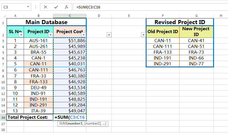
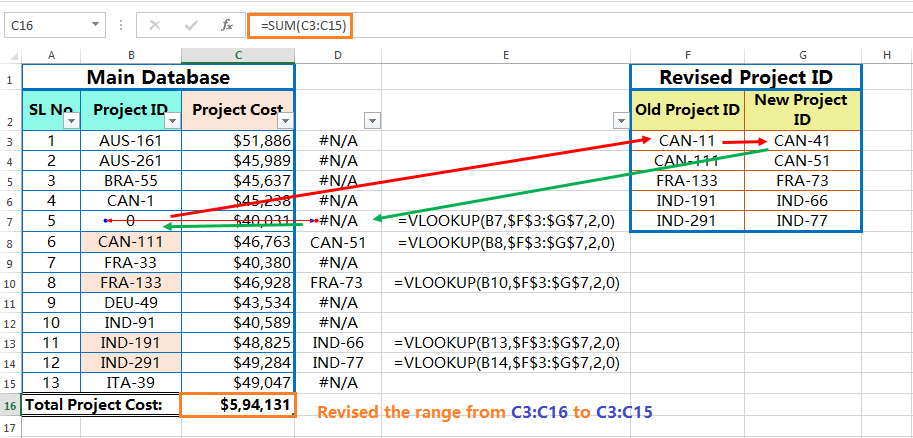
For example, we want to find out the sum of the Project Cost mentioned in column C. So in that case, we simply use the SUM formula in cell C16 and the SUM_range would be C3:C15. But unfortunately, if we extend the SUM_range downward to C3:C16, it creates a circular reference because the SUM formula in cell C16 refers to cell C16. Every time the SUM formula in C16 is calculated because the summation value in C16 has been changed. The calculation continues forever.

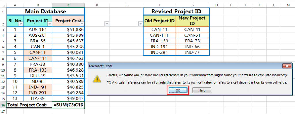
When we get the circular reference message after entering a formula, Excel gives two options:

• Either, click ‘OK‘, Excel returns a 0 (zero) value.

• Or, click on ‘Help’, Excel displays a Help screen that tells more about circular references.

II. WHAT IS AN INDIRECT CIRCULAR REFERENCE IN EXCEL?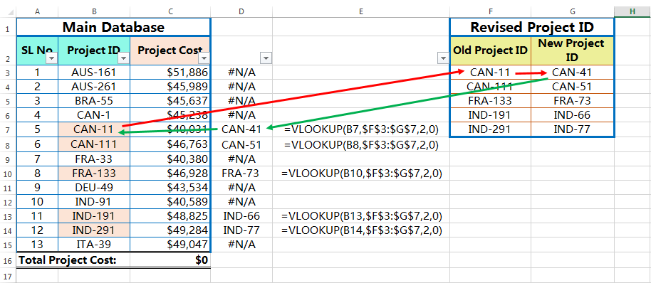

When a formula in a cell indirectly refers to its own cell is called an indirect circular reference.

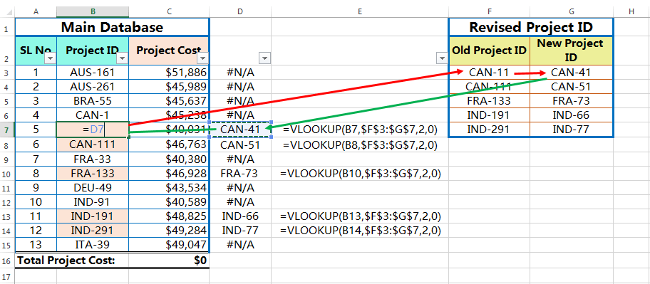
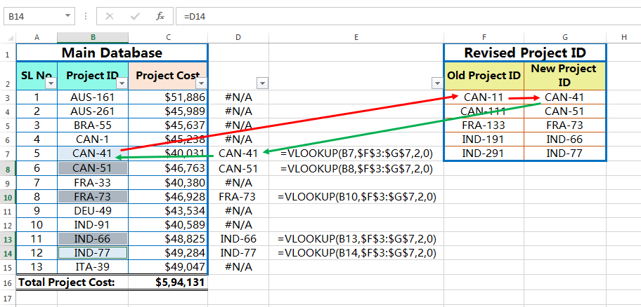
In the given example, we want to retrieve the data from ‘Revised Project ID’ to our ‘Main database’. So in that case, we commonly apply the VLOOKUP function to retrieve the exact match value. The VLOOKUP function is applied in column D, just beside the main database.

As a result, ‘New Project ID’ has been mapped against the ‘Old Project ID’ in column D. If we want to replace the New Project ID (i.e., the value of column D) on the Old Project ID (i.e., on column B) using the cell reference (with the equality ‘=’ sign), it creates a circular reference and Excel returns a 0 (zero) value. In detail, the formula in cell B7 directly refers to the cell D7 which indirectly refers to its own cell, i.e., B7 (through the VLOOKUP function). Excel cannot allow this.

Note: (i) In many cases, when entering more than one formula with a circular reference, Excel doesn’t display the warning message repeatedly.

(ii) When we open the file again after saving then it also shows the warning message that one or more formula contains a circular reference. Always take care of the warning and check that circular reference is enabled.

III. VALUE ERROR IN EXCEL

When Excel cannot evaluate a formula correctly, it returns an error value. All Excel errors begin with a hash mark or pound sign (#).

Formulas may return an error value if a cell that they refer to has an error value. This is known as the ripple effect: A single error value can make its way to lots of other cells that contain formulas that depend on that cell.

There are a number of different error values displayed depending on the type of error:

Error	Reasons	Solution
#DIV/0!	The formula is trying to divide a value by zero or an empty cell.	Put a value in the cell.
#N/A	This error can mean a number of things, depending on the formula. Such as: (i) The formula refers (directly or indirectly) to a cell that uses the NA when data is not yet available. Excel’s charting features simply ignore #N/A where data is not available, so it is often useful to use #N/A when charting the data. If we were to simply leave the cell blanks, Excel would interpret the cells as a 0 value and distort the chart. (ii) This error also occurs if a lookup function (VLOOKUP, HLOOKUP, or MATCH) does not find a match. (iii) The Excel Function is missing one or more required arguments.	(i) Check to make sure the formula references the correct value. (ii) Make sure the lookup column in the dataset contains lookup criteria or not. (iii) Check all the required arguments in the function are mentioned or not.
#NAME?	The NAME error occurs if Excel cannot evaluate a defined name used in the formula. The name may not exist, may have been inadvertently deleted, or may be misspelled. For example, (i) Misspelled or invalid or function name, such as =VLOKUP instead of =VLOOKUP (ii) Parentheses missing from function, such as =TODAY instead of =TODAY() (iii) Omitted quotation marks around text, such as using text instead of “text” in the function =IF(A1=”text”, A1, ” “) (iv) Missing colon in a range reference, such as =SUM(A1A10) instead of =SUM(A1:A10)	(i) Make sure the name referenced is correct. (ii) Check all the parenthesis in the function. (iii) Make sure the mentioned text in the function should be in the double quotation mark. (iv) Make sure that the colon is present in a range reference.
#NULL!	Incorrect range separator, such as using a semicolon instead of a colon within a reference to a range. The NULL error signifies that no intersection exists for the ranges identified in the formula. For example, if we forget to put an operator between cell references, such as forgetting to put one of the plus signs in a formula such as = B3 + C3 D3
#NUM!	This error indicates that there is a problem with a number – either the number cannot be interpreted because it is too small or too big, or because it does not exist. Sometimes we have entered an invalid numeric value in a formula or a function, for example, when we specify a negative number where a positive number is expected.	Check the function for an unacceptable argument.
#REF!	The formula contains a reference to a cell that was deleted or replaced with other data. That means this error indicates a problem with a cell reference and is most often due to deleting rows, columns, or cells that were used in a formula.	Correct cell references
#VALUE!	The incorrect type of data used in an argument, such as referring to a cell that contains text instead of a value. The value error is also associated with entering incorrect arguments for an Excel function.	Double-check arguments and or operands.
######	The cell is not wide enough Widen the column width.	Widen the column width.

IV. HOW TO FIND CIRCULAR REFERENCE IN EXCEL?

To find the circular reference in Excel, we can follow any of the following 02 methods:

➢ Method 1: Press Ctrl+` (grave accent key) which will display cell formulas.

➢ Method 2: Go to the ‘Formulas‘ tab ➪ Click on the ‘Error Checking‘ drop-down menu under the Formula Auditing group ➪ click on ‘Circular References‘.

This command displays a list of all cells that are involved in the circular reference in Excel. Start by selecting the first cell listed and then sorted out the problem.

Note: Until we resolve a circular reference, the status bar indicates the location of a circular reference, such as Circular References: B7.

• Formula Auditing in Excel

Formula Auditing is a set of tools in Excel that enable users to display or trace relationships for formula cells, show formulas, check for errors, and evaluate formulas. Users can audit a workbook with the help of the Formula Auditing group on the Formulas tab. Auditing is especially useful in determining why an error occurs.

A. Trace Precedents and Dependents

Although Excel displays error messages, we might not know which cell is causing the error. Even if the worksheet does not contain errors, we can use formula auditing tools to identify which cells are used in formulas. Formulas involve both precedent and dependent cells. As an example, suppose we use the formula =B1+C1, which is located in cell A1.

Dependent cells depend on another cell to generate their values. In the case of our formula, cell A1 depends on the values in cells B1 and C1. Therefore, cell A1 is dependent on both
B1 and C1.

Precedent cells precede another cell that means Precedent cells are cells that are referenced by a formula in another cell. For example, in our formula, cells B1 and C1 precede cell A1. In other words, in order to determine the results of A1, we must first determine the values in B1 and C1. Therefore, both B1 and C1 are precedent cells.

Excel’s Formula Auditing tools trace both dependent and precedent cells. The tracer arrows, colored lines that show the relationship between precedent and dependent cells. The tracer starts in a precedent cell with the arrowhead ending in the dependent cell. The tracer arrows help us identify cells that cause errors. Blue arrows show cells with no errors. Red arrows show cells that cause errors.

If we double-click any of the tracer arrows, the cell at the other end will be selected.

➢ To Trace Dependents Excel, Complete the following steps:

First, select the cell that contains the formula for which we want to audit dependent cells ➪ Click the Formulas tab ➪ Click Trace Dependents in the Formula Auditing group.

➢ To Trace Precedents Excel, Complete the following steps:

Select the cell that contains the formula for which we want to audit precedent cells ➪ Click the Formulas tab ➪ Click Trace Precedents in the Formula Auditing group.

Note:

⇒ We cannot audit a range of cells at one time. We must audit each of the cells individually. Also, we cannot audit formulas on protected worksheets; we must unprotect the worksheet first.

⇒ Excel’s formula auditing tools cannot trace precedents or dependents in cases where a formula references values in text boxes, embedded charts, or pictures.

⇒ In addition, the formula auditing tools cannot be used with pivot tables or references that depend on the name constants.

TIP: GREEN TRIANGLE

Excel detects potential logic errors even if the formula does not contain a syntax error. For example, Excel might detect that =SUM(A2:A10) contains a potential error if cell A1 contains a value, assuming the possibility that the function might need to include A1 in the range of values to add. When this occurs, Excel displays a green triangle in the top-left corner of the cell. Click the cell containing the green triangle and click the error icon, the yellow diamond with the exclamation mark, to see a list of options to correct the error.

B. Remove Tracer Arrows

To remove tracer arrows, we can follow any of the 02 methods:

➢ Method 1: Go to the ‘Formulas‘ tab ➪ Formula Auditing group ➪ click the ‘Remove Arrows‘.

➢ Method 2: Go to the ‘Formulas‘ tab ➪ Formula Auditing group ➪ click the ‘Remove Arrows‘ drop-down ➪ select any of the options Remove Arrows, Remove Precedent Arrows, or Remove Dependent Arrows.

C. Error Checking & Repair Errors

When the tracing of precedents or dependents shows errors in formulas, or if we want to check for errors that have occurred in formulas anywhere in a worksheet, we can click Error Checking in the Formula Auditing group on the Formulas tab. The Error Checking dialog box opens.

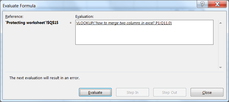
Click Help on this error to see a description of the error. But click Show Calculation Steps to open the Evaluate Formula dialog box, which provides an evaluation of the formula and shows which part of the evaluation will result in an error.

Clicking Ignore Error either moves to the next error or indicates that Error Checking is complete. When clicking Edit in Formula Bar, we can correct the formula in the Formula Bar.

V. HOW TO FIX CIRCULAR REFERENCE IN EXCEL?

If Excel displays an error message warning with a circular reference in Excel, we should fix it immediately. Unresolved circular references will cause unpredictable and inaccurate results in the working worksheet.

➢ Method 1: Using the Evaluate Formula dialog box

It is difficult to evaluate a nested formula due to the presence of intermediate calculations and logic tests. We can use the Evaluate Formula dialog box to view different parts of a nested formula and evaluate each part.

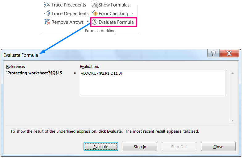
Select the cell we want to evaluate ➪ Click the Formulas tab ➪ Click Evaluate Formula in the Formula Auditing group to display the Evaluate Formula dialog box ➪ Click Evaluate to examine the value of the reference that is underlined ➪ Click Step In to display the other formula in the Evaluation box if the underlined part of the formula is a reference to another formula ➪ Click Step Out to return to the previous cell and formula.

Continue clicking Step In and Step Out until we can evaluate the entire formula and finally click Close.

➢ Method 2: Changing the Range

In the first case (Direct Circular Reference), change the range inside the SUM formula from C3:C16 to C3:C15. The circular reference has been fixed and the SUM formula returns the correct result.

➢ Method 3: Using the Paste Special dialog box

In the second case (Indirect Circular Reference), while we get the Circular Reference warning message at the beginning, we should try to escape (press the Esc key) and undo the process (with Ctrl+Z).

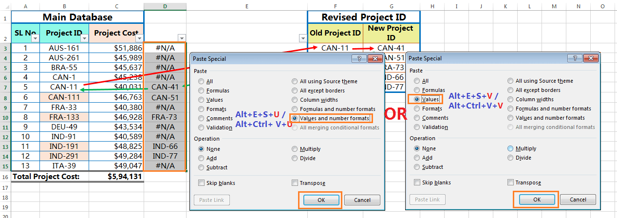
First, we make a copy of the formula range D3:D15 by Ctrl+C. Then convert the range of formulas to ‘values‘ using the Excel shortcut Alt+E+S+V (sequentially press Alt, E, S, V) or using another Excel shortcut Alt+Ctrl+V+V (sequentially press Alt+Ctrl+V, V). Similarly, we can convert the range of formulas to the ‘Values and number formats‘ with the Excel shortcut Alt+E+S+U (sequentially press Alt, E, S, U) or Alt+Ctrl+V+U (sequentially press Alt+Ctrl+V, U).

After that, we use a cell reference to get value from cell D7 to B7 (by using an equality ‘=’ sign). Then copy and paste the formula in B8, B10, B13, and B14 respectively.

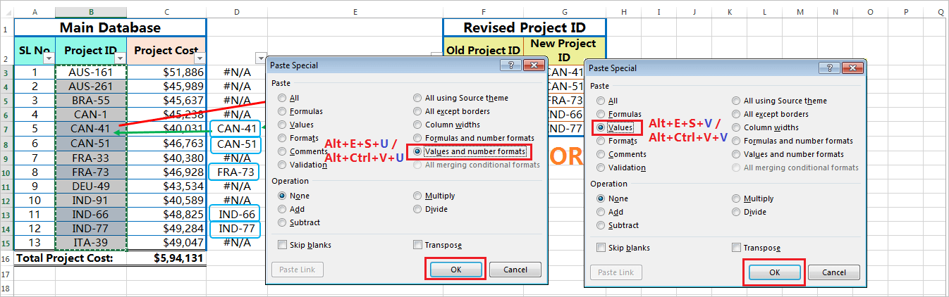
At last, copy the range B3:B15 and convert the range of formulas to ‘values‘ using Excel shortcut Alt+E+S+V (sequentially press Alt, E, S, V) or using another Excel shortcut Alt+Ctrl+V+V (sequentially press Alt+Ctrl+V, V). Similarly, convert the range of formulas to the ‘Values and number formats‘ with the Excel shortcut Alt+E+S+U (sequentially press Alt, E, S, U) or Alt+Ctrl+V+U (sequentially press Alt+Ctrl+V, U).

The above process fixes the indirect circular references and the Old Project IDs are successfully replaced by the new Project IDs.

If you would like to improve your academic and professional career as well, then the below courses help you a lot. Instead of Advanced Excel, a number of best courses suggested you through this platform that boosts your confidence and flies your career high.